Hello everyone. Last time, I wrote about “Thorough utilization of data that is sleeping in your company” as “Problem Solving Practice Edition”. In the post, I wrote that I would like to write about “Logistic Regression Analysis” later. So this time, I would like to write about it.
What is “Logistic Regression Analysis”?
In the previous post, I was trying to do multiple regression analysis using the following data.
Gender
Age
Age group
Marriage status
Living prefecture
Private brands you are aware of (multiple choice)
Image by private brand (multiple choice)
Change in purchase frequency of private brands in the last 1-2 years (increase/decrease/no change)
Reasons for the above (free answer)
Food products that have switched to private brands within the past year (multiple choice)
Seasonings that have switched to private brands within the past year (multiple selections)
Beverages that have switched to private brands within the past year (multiple choice)
Drugs that have switched to private brand within the past year (multiple choice), etc.
Looking at the raw data columns above, the first thing that seems to be the outcome variable is “Change in purchase frequency of private brands in the last 1-2 years (increase/decrease/no change). Also, it seems that “Foods/seasonings/beverages/drugs that have switched to private brand within the past year” can also be used.
“Changes in purchase frequency of private brands in the last 1-2 years (increased/decreased/no change)” are (1/2/3), “Foods/seasonings/beverages/drugs that have switched to private brand within the past year” is a multiple-choice answer (0/1). These types of data are called “discrete variables”.
Last time, I wanted to do a multiple regression analysis on Excel, so I made a column of continuous variables from discrete variables and proceeded with the analysis. Multiple regression analysis on Excel is called “linear regression analysis”, and only continuous variables can be taken as result variables, right?
This time, I will take up “logistic regression analysis” that can analyze the above discrete variables as outcome variables as they are.
Difference between “Multiple Regression Analysis” and “Logistic Regression Analysis”
In multiple regression analysis (linear regression analysis), the independent variable x changes the value of the outcome variable y. Therefore, it is possible to predict the “value” of the outcome variable from the independent variables. On the other hand, the result variable of logistic regression analysis is a discrete variable, so it is in the form of “1/0” (presence or absence of a specific phenomenon). That is, determine the probability that y would be 1. When multiple regression analysis (linear regression analysis) is used when the outcome variable is a discrete variable, there is nothing that cannot be analyzed, and I think that it will often output results that seem to be appropriate, but it is not always the correct result. So we should be careful.
Now, let’s perform a logistic regression analysis using “Changes in purchase frequency of private brand in the last 1-2 years (increased/decreased/no change)” as outcome variables.
Procedure of “Logistic Regression Analysis”
Unlike multiple regression analysis (linear regression analysis), logistic regression analysis cannot be performed in Excel, so this time we will use the statistical tool “R (free tool)” that can also perform logistic regression analysis. R is also a very useful tool that can handle various data mining (statistical analysis) methods such as multiple regression analysis (linear regression analysis), decision tree analysis, and cluster analysis. If you google R itself, you will find many articles, so I won’t write about it here (Let me put just one link here).
There are various ways to use R, but this time, I would like to proceed with the method of moving R by using “Google Colaboratory (Hereafter, “Colabo”. This is also free!)”. If you google about “Colabo” itself, you will find many articles, so I won’t write about it here (Let me put just one link here).
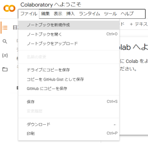
After accessing Colabo, first go to “File” -> “New Notebook” on the menu bar. *The screenshots are in Japanese, sorry.

Then proceed with “File” -> “Download” -> “Download .ipynb” on the menu bar.

Open the downloaded “.ipynb” file on text editors like Notepad, etc.

In the red squared part, update “name”: “python3”, “display_name”: “Python 3” as “name”: “ir”, “display_name”: “R” and save.

Go back to Colabo screen, and proceed with “File” -> “Upload notebook”, and choose the “.ipynb” file saved above.

Select “Runtime” → “Change runtime type” on the menu bar.

In the displayed dialog box, if “Runtime type” is “R”, it is OK. Now you are ready to run R on Colab.

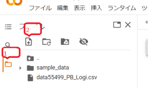
First, load the data file to be analyzed. Click the folder mark on the left side of the screen (callout 1 in Figure 8), then click the up arrow (callout 2 in Figure 8) to select the file.

Once the file is loaded, it’s time to run the logistic regression analysis.

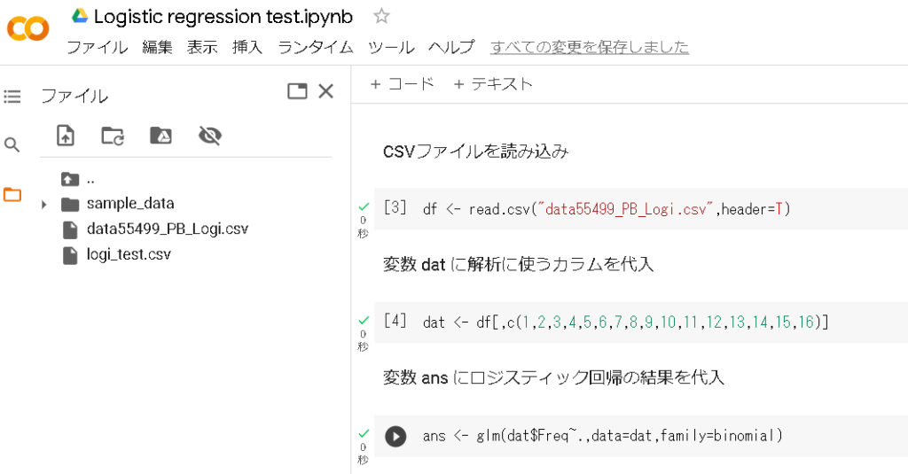
What I am doing in Figure 9 is as follows.
1. Read the data (CSV file loaded onto R) into the variable “dat (variable name can be anything)”
2. Specify the columns to be used for analysis from the data loaded in 1.
3. Execution of logistic regression analysis (“glm” on the right is the logistic regression analysis command. Here, the execution result is read into the variable “ans”)
How to understand the results
Now let’s view the analysis results.

In the middle, there is a table labeled “Coefficients:”. From left to right, ”Estimate”, ”Std.Error”, ”z value”, ”Pr(>|z|)”. The “Estimate” in this table is the same as the “Coefficient” in the multiple linear regression analysis, and “Pr(>|z|)” corresponds to the “P value”. The way of viewing these is the same as in multiple linear regression analysis, with P-values less than 5% and larger coefficients having a greater impact on the outcome variable. By looking at this result, the impact is larger in order of “Price (what to pay attention to when purchasing a private brand – [price])” and “Foods (the number of foods that have been switched to private brands within the past year)”.
Now for the logistic regression analysis, we need one more step. In case of multiple regression analysis, you create the formula Y=ax1+bx2+cx3…+d. Since Y was the outcome variable, we were able to predict Y by changing the coefficients (a,b,c in the above formula).
For logistic regression analysis, the outcome variable is a discrete variable and has the form 1/0. So, we have to think about the percentage of the result would become 1. Expressed as a formula, it looks like this.
log(p/1-p) =ax1+bx2+cx3…+d
p is the percentage of becoming 1 and 1-p is the percentage of not becoming 1. This ratio is called the odds ratio. I’m sure many of you have heard of it (reference, link). Logistic regression analysis models the impact of each independent variable on this odds ratio.
Now let’s use R to calculate the impact of each independent variable on this odds ratio.

Exp is a command that outputs the odds ratio, and as its parameter, we put in the variable containing the results of the logistic regression analysis earlier. As before (see Figure 10 above), from the left, there are ”Estimate”, ”Std.Error”, ”z value”, and ”Pr(>|z|)”, but the numbers are different. The number in this “Estimate” column is the size of the impact on the odds ratio.
As before, “Price (what to pay attention to when purchasing a private brand – [price])” and “Foods (the number of foods that have been switched to private brands within the past year)” have the greatest impact in that order. However, this time we can use these numbers as they are. Price is 2.43.., so if this variable increases by 1, the percentage (odds ratio) of “whether or not the frequency of private brand purchases has increased” is 2.43 times, and the same for Foods is 2.29 times.
That’s all for the logistic regression analysis. Although it requires one more task than linear multiple regression analysis, it can be performed with a free tool (Colabo & R), and if you learn this, you will be able to handle both continuous and discrete variables as outcome variables. Please try to add to your repertoire!
That’s all for this time, and I would like to continue from the next time onwards. Thank you for reading until the end.