Hello everyone. This time is also “Problem Solving Practice Edition”. This time, I would like to take up “Thorough utilization of data that is sleeping in your company”. Throughout my career, I have often heard people say, “We have a lot of data, but we haven’t been able to use it at all.” Also, I have seen many results of customer surveys that I do not know who is using it for what, even in the companies I have actually belonged to. This time, I would like to introduce an example of how to use such “sleeping data”.
Example of common survey results
As a theme for this time, I searched for open data that summarizes the so-called basic aggregation results and that allows the raw data of the aggregation to be downloaded. This kind of open data is published by many major research companies. Among them, I found this open data (survey results on “private brand”). Let’s take a look at some of these results.

First, this survey asked about the increase or decrease in the frequency of purchasing private brand products. If you look at this, I think you can read as “Most people haven’t changed.”
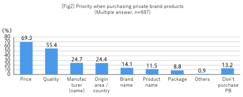
Next, the survey asked about important factors when purchasing private brand products. Looking at this, I think you can read as “Price is important”, “But the majority pointed out the quality as well. So quality is also important”.
What do you think? I don’t think it will be denied because it probably doesn’t deviate from the feeling of many people, but I also don’t think that people say “I see!”. And it feels that the results would be perceived as “Hmm, that’s right”, and it would go into “sleeping” mode.
(Caution) I would like to add that I don’t have any intention to disrespect this research company by all means and that there are many research companies that who publish only common contents as the open data and in-depth analysis is separately consulted.
Thorough utilization of data
Check raw data
Now let’s check the contents of the raw data to make full use of the data.
Gender
Age
Age group
Marriage status
Living prefecture
Private brands you know (multiple choice)
Image by private brand
Change in purchase frequency of private brands in the last 1-2 years (increase/decrease/no change)
Reasons for the above (free answer)
Food products that have switched to private brands within the past year (multiple choice)
Seasonings that have switched to private brands within the past year (multiple selections)
Beverages that have switched to private brands within the past year (multiple choice)
Drugs that have switched to private brand within the past year (multiple choice), etc.
In this type of case, first “multiple regression analysis”!
If you find data with many columns, such as the customer survey results above, try multiple regression analysis first! *Decision tree analysis is also good. I would like to write about decision tree in the future (I wrote it! -> here).
The first thing to consider in multiple regression analysis is what should be the outcome variable and what should be the independent variable. The outcome variable is the result of some activity, such as “Revenue” or “Customer Satisfaction”. Independent variables are variables for predicting the “outcome”.
Looking at the raw data columns above, the first thing that seems to be the outcome variable is “Change in purchase frequency of private brands in the last 1-2 years (increase/decrease/no change). Also, it seems that “Foods/seasonings/beverages/drugs that have switched to private brand within the past year” can also be used.
Now let’s take a look at the data in those columns.

“Changes in purchase frequency of private brands in the last 1-2 years (increased/decreased/no change)” are (1/2/3), “Foods/seasonings/beverages/drugs that have switched to private brand within the past year” is a multiple-choice answer (0/1). These types of data, which are numbers, but are just numbers assigned to options, do not represent size, and are meaningless to calculate are called “discrete variables”. It’s a name that’s unique to statistics and difficult to get used to, but let’s just memorize it.
Contrary to discrete variables, data types that that have large and small in them and are meaningful to calculate are called “continuous variables”. Note that these data type differences affect the available statistical methods.
And, as mentioned above, when the outcome variable is a “discrete variable”, a method called “logistic regression analysis” is used in multiple regression analysis (I would like to write about logistic regression analysis in this blog later -> I wrote it!). The multiple regression analysis that is usually used in Excel is actually a slightly different method called “linear regression analysis”. In fact, even if the outcome variable is a “discrete variable”, there is no reason why it cannot be analyzed by “linear regression analysis”, but let’s proceed according to theory here.
Then, even if you look at the above raw data, it seems that there is no “continuous variable” that can be the outcome variable as it is. It’s a problem solver’s value to add a little twist here lol. Looking at Figure 3 above, “Foods/seasonings/beverages/drugs that have switched to private brand within the past year” is a discrete variable (0/1) for each product. By totaling these horizontally, it is possible to create a new continuous variable column of “number of foods/seasonings/beverages/pharmaceuticals switched to private brands within the past year”. Let’s proceed with multiple regression analysis using this as the outcome variable.
As for the independent variables, it doesn’t matter if they are “discrete variables” or “continuous variables”. however, note that “discrete variables” must always be in the form (0/1).
Data shaping
Then, based on the above policy, let’s shape the raw data for multiple regression analysis.
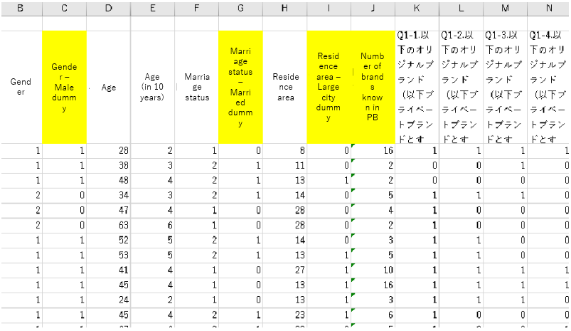
First is the independent variables. Column B “Gender” in Figure 4 is (1=male, 2=female). Here we want to set it to (0/1), so create a dummy column called “gender – male dummy” in column C, and if column B is “1”, it will be “1”, and if column B is “2” It is converted to put “0”. Similarly, column F “Marriage status” is also (1=unmarried, 2=married), so a dummy column is created in column G and converted to (1=married, 0=unmarried).
Column H, “Living prefecture,” contains large numbers, but this is actually 47 prefectures. We would like to set this to (0/1) as well, so here I created a dummy column called “Residence – large city dummy” in column I and set it as (1 = Tokyo, Aichi, Osaka, Fukuoka, 0 = other). In addition, since columns K to AB list individual private brand names in the form of (1 = known, 0 = unknown), I created a dummy column called “Number of brands known in PB” in column J and added the horizontal sum of columns K to AB in the column.
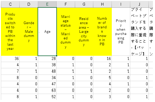
After data shaping, it looks like the above. Column C is the outcome variable, and as explained above, it is a newly created continuous variable column that says “the number of products that have switched to private brand within the past year”. This time, food/seasoning/beverage/drugs are all added up as the “number of products”.
The independent variables are the dummy columns described above, plus the “Age” in column E is a continuous variable, so I left it as is. In addition, columns I to O, “Priority when purchasing PB,” are discrete variables (0/1), so they are left as they are.
Analysis
Two important preparations before the analysis were “handling missing values” and “multicollinearity check”, right? There were no “missing values” in the data this time, so it was okay. Then, let’s also check “multicollinearity”. The first is correlation analysis.
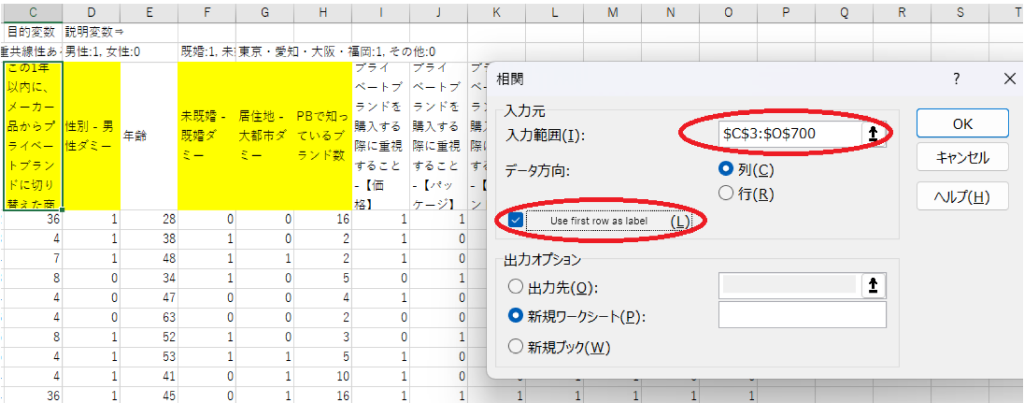
Proceed with the formatted data in Figure 5. Select “Data” -> “Data Analysis” from the Excel menu bar and select “Correlation” from the dialog box.

Next, specify the range of the data shaped in Fig. 5 in “Input Range” in the “Correlation” dialog box. Check “Use first row as labels” so that analysis results are easier to see.
Like this, each correlation coefficient is output in the lower left half, and the upper right half is blank. Fill in the upper right half by copying each correlation coefficient and pasting it with “Transpose”.

Create a new table by copying the vertical and horizontal axes of the correlation coefficient table created in Figure 8. The inverse matrix is automatically entered in the inner part of the table by using the function “minverse”. Each diagonal cell from the upper left to the lower right of this inverse matrix table is the Value Inflation Factor (VIF). The part where this VIF exceeds 10 (red in Fig. 9) is the part with multicollinearity. The relevant columns here, in this example “Age” and “age in 10 years”, one of which will be retained and the other will be removed. This time, we will leave the “age” and proceed.

Now let’s do a multiple regression analysis! Proceed with the formatted data in Figure 5. As in Figure 6, select “Data” -> “Data Analysis” from the Excel menu bar, and select “Regression Analysis” from the dialog box this time.
Next, in the “Regression Analysis” dialog box, specify column C which is the outcome variable in “Input Y Range” and the remaining columns in “Input X Range”. Also check the “Label” so that analysis results are easier to see.

Familiar (lol), the regression analysis result of Excel came out (Fig. 11). There were three points to see in this, right?
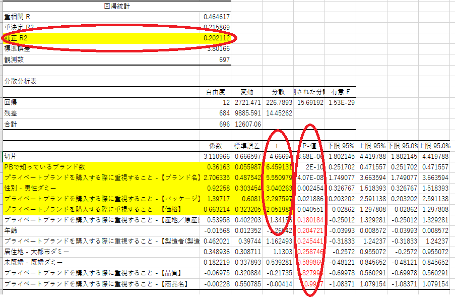
First of all, “Adjusted R2” is about 20% this time. This means that about 20% of the increase or decrease in the outcome variable, “the number of products that have been switched to private brands within the past year,” can be explained by the independent variables included in this analysis. Of course, the closer to 100% is the better, so it may look small, but I think in many cases when analyzing using actual data from business sites, the number would be around here. If you can explain even 10%, I think you can say that there is enough suggestion.
Then sort the “P-value” column in ascending order and only focus on the independent variables that are less than 5%. Finally, sort the “t” column in descending order, only for the independent variables we focused on. If “t” is 2 or more, it should be focused. This time, the “t” of the independent variables with “P-value” less than 5% were all 2 or more, so it can be said that these independent variables have a statistically large impact on the outcome variable.
Number of brands known in PB
Priority when purchasing PB – [Brand name]
Gender – Male dummy
Priority when purchasing PB – [Package]
Priority when purchasing PB – [Price]
After all, “price” is also included, but it can be seen that the elements such as “brand awareness”, “brand name”, and “package” are more important than that.
Summary
If we recall the aggregate results in Fig. 2 at the beginning, we saw that “Price is important”, “But the majority pointed out the quality as well. So quality is also important”, right? It is true that there are many people who say Quality is important based on simple aggregation, but it turns out that it is not the case that those people are actually switching to private brands.
What did you think? I think I have conveyed to you that the company’s “dormant data” can also be used to “focus” the strategy by trying to analyze it with a little ingenuity like this time.
That’s all for this time, and I would like to continue from the next time onwards. Thank you for reading until the end.